Climate-PINN: Model Architecture

PINN Architecture Overview

The Climate-PINN combines neural network components with physics-based constraints to create a model that respects fluid dynamics while making accurate predictions.

The overall architecture of the Climate-PINN model

Key Components

MeteoEncoder

CNN-based encoder that processes meteorological input variables:

Geopotential at 500 hPa
Temperature at 850 hPa

Uses convolutional layers with non-linear activations to extract spatial features.

MaskEncoder

Processes geographical constraints:

Orography (terrain elevation)
Land-sea mask
Soil type

Helps the model understand how geography affects climate patterns.

CoordProcessor

Handles coordinate information:

Latitude and longitude
Temporal coordinates

Enables the model to understand spatial and temporal relationships.

Feature Combiner

Integrates features from all encoders:

Concatenates features from different branches
Processes combined features through CNN layers
Outputs prediction for temperature and wind components

Physics Constraints

What makes Climate-PINN unique is its incorporation of fluid dynamics principles from the Navier-Stokes equations directly into the learning process.

Continuity Equation

$$\nabla \cdot \mathbf{u} = 0$$

Ensures conservation of mass in the fluid flow.

Momentum Equations

$$\frac{\partial \mathbf{u}}{\partial t} + (\mathbf{u} \cdot \nabla)\mathbf{u} = -\nabla p + \frac{1}{Re}\nabla^2\mathbf{u}$$

Govern the conservation of momentum in x and y directions.

Reynolds Number

$$Re = \frac{\rho u L}{\mu}$$

The model learns an appropriate Reynolds number to balance inertial and viscous forces.

Physics-Informed Loss Function

The total loss combines traditional data-driven loss with physics constraint residuals:

$$L_{total} = L_{data} + \lambda_{physics} \times L_{physics}$$

Where $L_{physics}$ includes residuals from continuity and momentum equations:

physics_loss = {
    'e1': self.MSE(e1, torch.zeros_like(e1)),  # Continuity equation
    'e2': self.MSE(e2, torch.zeros_like(e2)),  # x-momentum
    'e3': self.MSE(e3, torch.zeros_like(e3))   # y-momentum
}

Model Variants

The repository includes several model variants with progressive improvements.

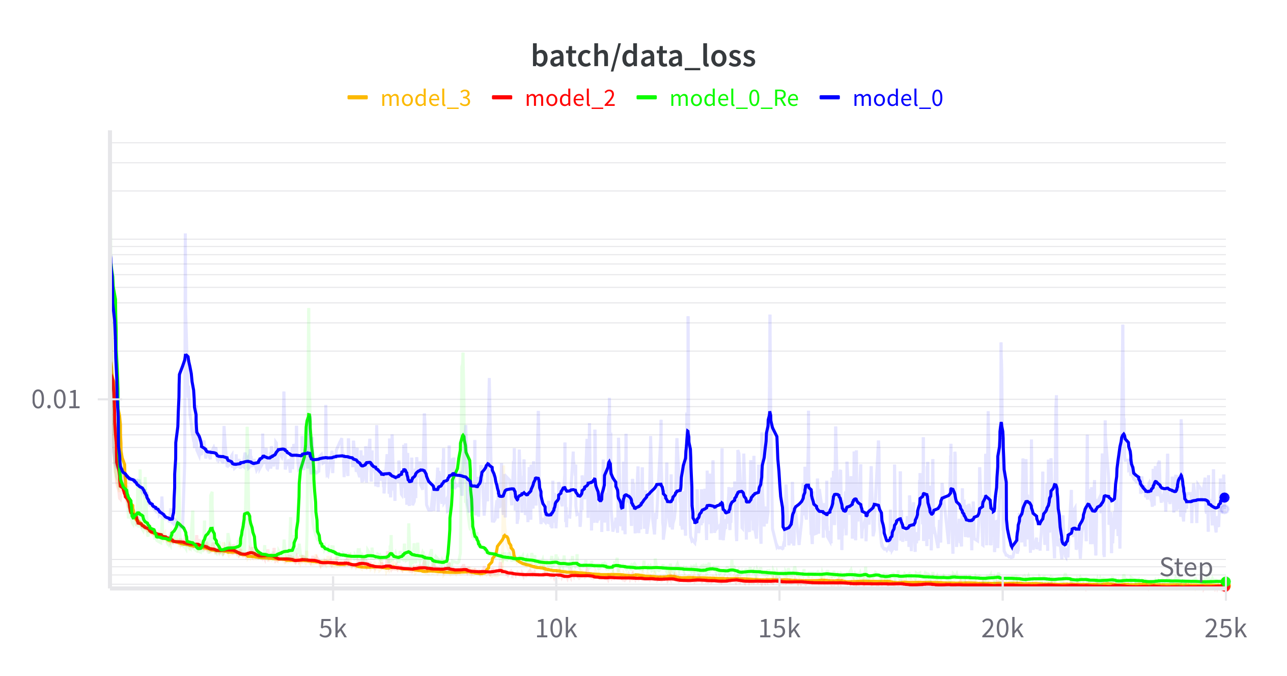
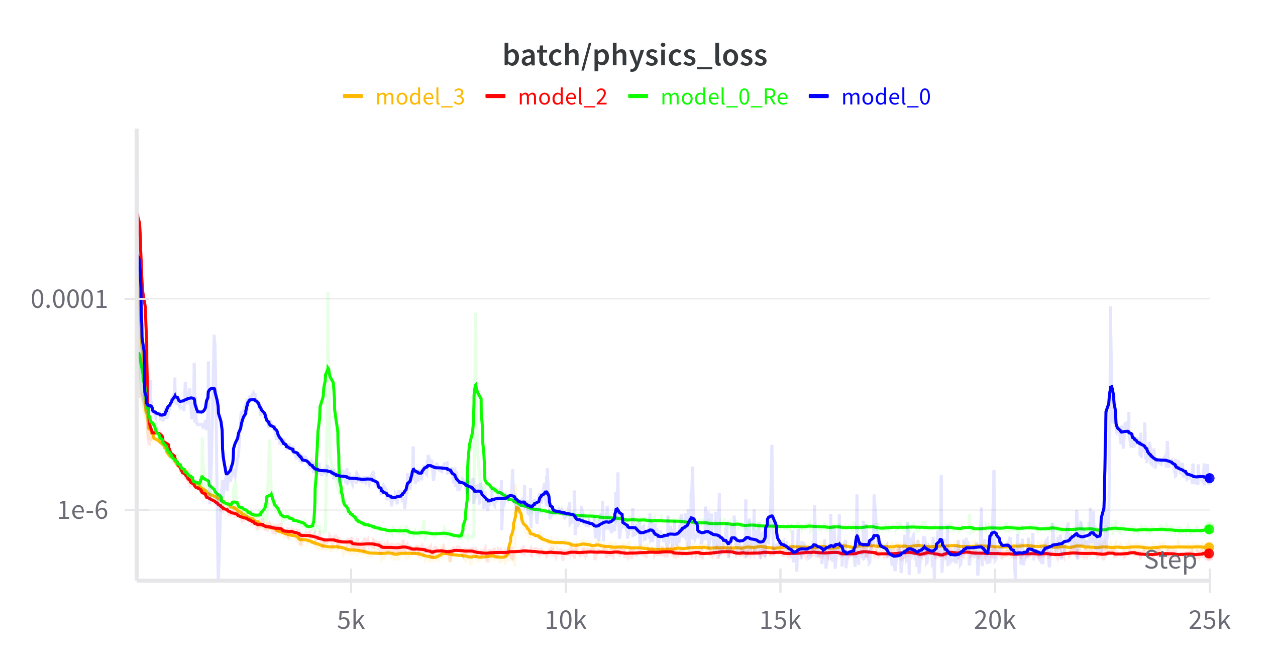
Model 0: Baseline

The original baseline model with basic architecture.

Key Features:

Basic encoder-decoder architecture
Simple physics constraints integration
No specialized handling of Reynolds number
Tanh activation functions

Architecture Diagram:

Model 0 Re: Enhanced Reynolds Number

Improved handling of the Reynolds number parameter with gradient clipping and momentum.

Key Improvements:

Clipped gradient for the Reynolds number
Momentum-based smoothing of Reynolds number updates
Added BatchNorm layers for stability
Constrained Reynolds number to physically meaningful range (50-1e5)

Reynolds Number Code:

def get_reynolds_number(self):
    clamped_log_re = torch.clamp(self.log_re,
                                min=torch.log(torch.tensor(50.0, device=self.device)),
                                max=torch.log(torch.tensor(1e5, device=self.device)))
    current_re = torch.exp(clamped_log_re)

    if self.previous_re is None:
        self.previous_re = current_re

    smoothed_re = self.re_momentum * self.previous_re + (1 - self.re_momentum) * current_re
    self.previous_re = smoothed_re.detach()

    return smoothed_re

Model 1: Modified Dropout

Introduction of dropout layers for improved generalization.

Key Changes:

Added dropout layers (p=0.2) for regularization
Positioning of dropout after activation functions
Maintained Tanh activation functions
No changes to Reynolds number handling

Note: This model has suboptimal dropout placement which was corrected in Model 2.

Model 2: Optimized Architecture

Significant architectural improvements including residual connections and proper dropout placement.

Major Enhancements:

Added residual connections (ResBlocks) for better gradient flow
Switched from Tanh to ReLU activations
Proper placement of dropout layers
Improved Reynolds number handling with clipping and momentum
Added BatchNorm for more stable training

ResBlock Implementation:

class ResBlock(torch.nn.Module):
    def __init__(self, in_channel):
        super().__init__()

        self.conv_block = torch.nn.Sequential(
                    torch.nn.Conv2d(in_channels=in_channel,
                            out_channels=in_channel,
                            kernel_size=3,
                            stride=1,
                            padding='same'),
                    torch.nn.BatchNorm2d(in_channel),
                    torch.nn.ReLU(),
                    torch.nn.Conv2d(in_channels=in_channel,
                            out_channels=in_channel,
                            kernel_size=3,
                            stride=1,
                            padding='same'),
                    torch.nn.BatchNorm2d(in_channel)
        )
        self.act = torch.nn.ReLU()

    def forward(self, input):
        out = self.conv_block(input)
        out += input
        out = self.act(out)
        return out

Model 3: Neural Network for Reynolds Number

Advanced model with a dedicated neural network for estimating the Reynolds number.

Key Innovations:

Neural network to predict spatially-varying Reynolds number
Reynolds number estimated from local flow conditions (u, v)
All improvements from Model 2 maintained
More physically realistic modeling of turbulence

Reynolds Network:

class ReynoldsNetwork(nn.Module):
    def __init__(self, hidden_dim=16):
        super().__init__()
        self.re_net = nn.Sequential(
            nn.Conv2d(2, hidden_dim, kernel_size=3, padding=1),
            nn.ReLU(),
            nn.Conv2d(hidden_dim, hidden_dim, kernel_size=3, padding=1),
            nn.ReLU(),
            nn.Dropout(p=0.2),
            nn.Conv2d(hidden_dim, 1, kernel_size=3, padding=1),
            nn.Sigmoid()  # Ensure positive output
        )

    def forward(self, u, v):
        inputs = torch.stack([u, v], dim=1)
        re = self.re_net(inputs)
        # Scale output to a reasonable range for Reynolds number
        re = re * (1e5 - 50.0) + 50.0
        return re

Model Performance Comparison

Comparison of different model variants across metrics:

MSE Loss

Model	Train	Val	Test	Average
model_0	0.0017	0.0017	0.0017	0.0017
model_1	0.0063	0.0063	0.0080	0.0069
model_0_Re	9.42e-04	9.62e-04	0.0016	0.0012
model_2	5.89e-04	6.51e-04	0.0012	8.22e-04
model_3	6.08e-04	6.57e-04	0.0013	8.48e-04

Physics Loss

Model	Train	Val	Test	Average
model_0	5.56e-07	5.83e-07	6.69e-07	6.03e-07
model_1	1.22e-07	1.79e-07	1.43e-07	1.48e-07
model_0_Re	6.08e-05	6.59e-05	6.11e-05	6.26e-05
model_2	3.29e-06	2.70e-06	3.51e-06	3.17e-06
model_3	5.04e-06	3.72e-06	5.50e-06	4.75e-06

Total Loss

Model	Train	Val	Test	Average
model_0	0.0017	0.0017	0.0017	0.0017
model_1	0.0063	0.0063	0.0080	0.0069
model_0_Re	0.0010	0.0010	0.0017	0.0012
model_2	5.92e-04	6.54e-04	0.0012	8.25e-04
model_3	6.13e-04	6.61e-04	0.0013	8.53e-04

MSE comparison across models

Physics constraint loss comparison

Model 2 demonstrates the best overall performance with the lowest MSE and total loss across all datasets, while Model 0 shows the lowest physics constraint violations. This suggests that Model 2 offers the best balance between data prediction accuracy and physics-informed constraints.

Pretrained Model Weights

Pretrained weights for all model variants are available on Hugging Face:

Download Model Weights

All models are trained on 10 years of ERA5 data with balanced physics and data loss weights.